Nested Resampling with rsample

A typical scheme for splitting the data when developing a predictive model is to create an initial split of the data into a training and test set. If resampling is used, it is executed on the training set where a series of binary splits is created. In rsample, we use the term analysis set for the data that are used to fit the model and the assessment set is used to compute performance:

A common method for tuning models is grid search where a candidate set of tuning parameters is created. The full set of models for every combination of the tuning parameter grid and the resamples is created. Each time, the assessment data are used to measure performance and the average value is determined for each tuning parameter.

The potential problem is, once we pick the tuning parameter associated with the best performance, this value is usually quoted as the performance of the model. There is serious potential for optimization bias since we uses the same data to tune the model and quote performance. This can result in an optimistic estimate of performance.

Nested resampling does an additional layer of resampling that separates the tuning activities from the process used to estimate the efficacy of the model. An outer resampling scheme is used and, for every split in the outer resample, another full set of resampling splits are created on the original analysis set. For example, if 10-fold cross-validation is used on the outside and 5-fold cross-validation on the inside, a total of 500 models will be fit. The parameter tuning will be conducted 10 times and the best parameters are determined from the average of the 5 assessment sets.

Once the tuning results are complete, a model is fit to each of the outer resampling splits using the best parameter associated with that resample. The average of the outer method's assessment sets are a unbiased estimate of the model.

To get started, let's load the packages that will be used in this post.

library(rsample)   
library(purrr)
library(dplyr)
library(ggplot2)
library(scales)
library(mlbench)
library(kernlab)
library(sessioninfo)
theme_set(theme_bw())

We will simulate some regression data to illustrate the methods. The function mlbench::mlbench.friedman1 can simulate a complex regression data structure from the original MARS publication. A training set size of 100 data points are generated as well as a large set that will be used to characterize how well the resampling procedure performed.

sim_data <- function(n) {
  tmp <- mlbench.friedman1(n, sd=1)
  tmp <- cbind(tmp$x, tmp$y)
  tmp <- as.data.frame(tmp)
  names(tmp)[ncol(tmp)] <- "y"
  tmp
}

set.seed(9815)
train_dat <- sim_data(100)
large_dat <- sim_data(10^5)

To get started, the types of resampling methods need to be specified. This isn't a large data set, so 5 repeats of 10-fold cross validation will be used as the outer resampling method that will be used to generate the estimate of overall performance. To tune the model, it would be good to have precise estimates for each of the values of the tuning parameter so 25 iterations of the bootstrap will be used. This means that there will eventually be 5 * 10 * 25 = 1250 models that are fit to the data per tuning parameter. These will be discarded once the performance of the model has been quantified.

To create the tibble with the resampling specifications:

results <- nested_cv(train_dat, 
                     outside = vfold_cv(repeats = 5), 
                     inside = bootstraps(25))
results

## # 10-fold cross-validation repeated 5 times 
## # Nested : vfold_cv(repeats = 5) / bootstraps(25) 
## # A tibble: 50 x 4
##          splits      id    id2   inner_resamples
##          <list>   <chr>  <chr>            <list>
##  1 <S3: rsplit> Repeat1 Fold01 <tibble [25 x 2]>
##  2 <S3: rsplit> Repeat1 Fold02 <tibble [25 x 2]>
##  3 <S3: rsplit> Repeat1 Fold03 <tibble [25 x 2]>
##  4 <S3: rsplit> Repeat1 Fold04 <tibble [25 x 2]>
##  5 <S3: rsplit> Repeat1 Fold05 <tibble [25 x 2]>
##  6 <S3: rsplit> Repeat1 Fold06 <tibble [25 x 2]>
##  7 <S3: rsplit> Repeat1 Fold07 <tibble [25 x 2]>
##  8 <S3: rsplit> Repeat1 Fold08 <tibble [25 x 2]>
##  9 <S3: rsplit> Repeat1 Fold09 <tibble [25 x 2]>
## 10 <S3: rsplit> Repeat1 Fold10 <tibble [25 x 2]>
## # ... with 40 more rows

The splitting information for each resample is contained in the split objects. Focusing on the second fold of the first repeat:

results$splits[[2]]

## <90/10/100>

<90/10/100> indicates the number of data in the analysis set, assessment set, and the original data.

Each element of inner_resamples has its own tibble with the bootstrapping splits.

results$inner_resamples[[5]]

## # Bootstrap sampling with 25 resamples 
## # A tibble: 25 x 2
##          splits          id
##          <list>       <chr>
##  1 <S3: rsplit> Bootstrap01
##  2 <S3: rsplit> Bootstrap02
##  3 <S3: rsplit> Bootstrap03
##  4 <S3: rsplit> Bootstrap04
##  5 <S3: rsplit> Bootstrap05
##  6 <S3: rsplit> Bootstrap06
##  7 <S3: rsplit> Bootstrap07
##  8 <S3: rsplit> Bootstrap08
##  9 <S3: rsplit> Bootstrap09
## 10 <S3: rsplit> Bootstrap10
## # ... with 15 more rows

These are self-contained, meaning that the bootstrap sample is aware that it is a sample of a specific 90% of the data:

results$inner_resamples[[5]]$splits[[1]]

## <90/37/90>

To start, we need to define how the model will be created and measured. For our example, a radial basis support vector machine model will be created using the function kernlab::ksvm. This model is generally thought of as having two tuning parameters: the SVM cost value and the kernel parameter sigma. For illustration, only the cost value will be tuned and the function kernlab::sigest will be used to estimate sigma during each model fit. This is automatically done by ksvm.

After the model is fit to the analysis set, the root-mean squared error (RMSE) is computed on the assessment set. One important note: for this model, it is critical to center and scale the predictors before computing dot products. We don't do this operation here because mlbench.friedman1 simulates all of the predictors to be standard uniform random variables.

Our function to fit a single model and compute the RMSE is:

# `object` will be an `rsplit` object from our `results` tibble
# `cost` is the tuning parameter
svm_rmse <- function(object, cost = 1) {
  y_col <- ncol(object$data)
  mod <- ksvm(y ~ ., data = analysis(object),  C = cost)
  holdout_pred <- predict(mod, assessment(object)[-y_col])
  rmse <- sqrt(mean((assessment(object)$y - holdout_pred)^2, na.rm = TRUE))
  rmse
}

# In some case, we want to parameterize the function over the tuning parameter:
rmse_wrapper <- function(cost, object) svm_rmse(object, cost)

For the nested resampling, a model needs to be fit for each tuning parameter and each bootstrap split. To do this, a wrapper can be created:

# `object` will be an `rsplit` object for the bootstrap samples
tune_over_cost <- function(object) {
  results <- tibble(cost = 2^seq(-2, 8, by = 1))
  results$RMSE <- map_dbl(results$cost, 
                          rmse_wrapper,
                          object = object)
  results
}

Since this will be called across the set of outer cross-validation splits, another wrapper is required:

# `object` is an `rsplit` object in `results$inner_resamples` 
summarize_tune_results <- function(object) {
  # Return row-bound tibble that has the 25 bootstrap results
  map_df(object$splits, tune_over_cost) %>%
    # For each value of the tuning parameter, compute the 
    # average RMSE which is the inner bootstrap estimate. 
    group_by(cost) %>%
    summarize(mean_RMSE = mean(RMSE, na.rm = TRUE),
              n = length(RMSE))
}

Now that those functions are defined, we can execute all the inner resampling loops:

tuning_results <- map(results$inner_resamples, summarize_tune_results) 

tuning_results is a list of data frames for each of the 50 outer resamples.

Let's make a plot of the averaged results to see what the relationship is between the RMSE and the tuning parameters for each of the inner bootstrapping operations:

pooled_inner <- tuning_results %>% bind_rows

best_cost <- function(dat) dat[which.min(dat$mean_RMSE),]

p <- ggplot(pooled_inner, aes(x = cost, y = mean_RMSE)) + 
  scale_x_continuous(trans='log2') +
  xlab("SVM Cost") + ylab("Inner RMSE")

for(i in 1:length(tuning_results))
  p <- p  + 
  geom_line(data = tuning_results[[i]], alpha = .2) + 
  geom_point(data = best_cost(tuning_results[[i]]), pch = 16)

p <- p + geom_smooth(data = pooled_inner, se = FALSE)
p

## `geom_smooth()` using method = 'loess'

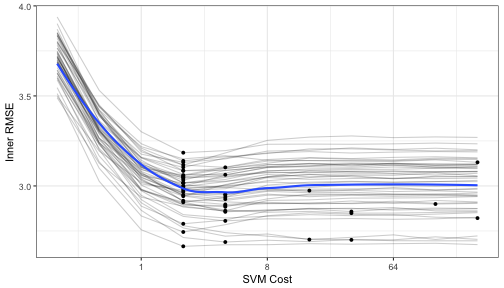
Each grey line is a separate bootstrap resampling curve created from a different 90% of the data. The blue line is a loess smooth of all the results pooled together.

To determine the best parameter estimate for each of the outer resampling iterations:

cost_vals <- tuning_results %>% map_df(best_cost) %>% select(cost) 
results <- bind_cols(results, cost_vals)

ggplot(results, aes(x = factor(cost))) + geom_bar() + xlab("SVM Cost")

Most of the resamples produced an optimal cost values of 2.0 but the distribution is right-skewed due to the flat trend in the resampling profile once the cost value becomes 10 or larger.

Now that we have these estimates, we can compute the outer resampling results for each of the 50 splits using the corresponding tuning parameter value:

results$RMSE <- map2_dbl(results$splits, results$cost, svm_rmse)
summary(results$RMSE)

##    Min. 1st Qu.  Median    Mean 3rd Qu.    Max. 
##   1.086   2.183   2.562   2.689   3.191   4.222

The RMSE estimate using nested resampling is 2.69.

What is the RMSE estimate for the non-nested procedure when only the outer resampling method is used? For each cost value in the tuning grid, 50 SVM models are fit and their RMSE values are averaged. The table of cost values and mean RMSE estimates is used to determine the best cost value. The associated RMSE is the biased estimate.

not_nested <- map(results$splits, tune_over_cost) %>%
  bind_rows

outer_summary <- not_nested %>% 
  group_by(cost) %>% 
  summarize(outer_RMSE = mean(RMSE),
            n = length(RMSE))
outer_summary

## # A tibble: 11 x 3
##      cost outer_RMSE     n
##     <dbl>      <dbl> <int>
##  1   0.25   3.565595    50
##  2   0.50   3.119439    50
##  3   1.00   2.775602    50
##  4   2.00   2.609950    50
##  5   4.00   2.639033    50
##  6   8.00   2.755651    50
##  7  16.00   2.831902    50
##  8  32.00   2.840183    50
##  9  64.00   2.833896    50
## 10 128.00   2.831717    50
## 11 256.00   2.836863    50

ggplot(outer_summary, aes(x = cost, y = outer_RMSE)) + 
  geom_point() + 
  geom_line() + 
  scale_x_continuous(trans='log2') +
  xlab("SVM Cost") + ylab("Inner RMSE")

The non-nested procedure estimates the RMSE to be 2.61. Both estimates are fairly close and would end up choosing a cost parameter value of 2.0.

The approximately true RMSE for an SVM model with a cost value of 2.0 and be estimated with the large sample that was simulated at the beginning.

finalModel <- ksvm(y ~ ., data = train_dat, C = 2)
large_pred <- predict(finalModel, large_dat[, -ncol(large_dat)])
sqrt(mean((large_dat$y - large_pred)^2, na.rm = TRUE))

## [1] 2.696096

The nested procedure produces a closer estimate to the approximate truth but the non-nested estimate is very similar. There is some optimzation bias here but it is very small (for these data and this model).

The R markdown document used to create this post can be found here.

The session information is:

session_info()

## ─ Session info ──────────────────────────────────────────────────────────
##  setting  value                       
##  version  R version 3.3.3 (2017-03-06)
##  os       macOS Sierra 10.12.6        
##  system   x86_64, darwin13.4.0        
##  ui       X11                         
##  language (EN)                        
##  collate  en_US.UTF-8                 
##  tz       America/New_York            
##  date     2017-09-03                  
## 
## ─ Packages ──────────────────────────────────────────────────────────────
##  package     * version  date       source         
##  assertthat    0.2.0    2017-04-11 CRAN (R 3.3.2) 
##  bindr         0.1      2016-11-13 CRAN (R 3.3.2) 
##  bindrcpp    * 0.2      2017-06-17 cran (@0.2)    
##  broom       * 0.4.2    2017-02-13 CRAN (R 3.3.2) 
##  clisymbols    1.2.0    2017-05-21 CRAN (R 3.3.2) 
##  colorspace    1.3-2    2016-12-14 CRAN (R 3.3.2) 
##  dplyr       * 0.7.2    2017-07-20 cran (@0.7.2)  
##  evaluate      0.10.1   2017-06-24 CRAN (R 3.3.2) 
##  foreign       0.8-67   2016-09-13 CRAN (R 3.3.3) 
##  ggplot2     * 2.2.1    2016-12-30 CRAN (R 3.3.2) 
##  glue          1.1.1    2017-06-21 CRAN (R 3.3.2) 
##  gtable        0.2.0    2016-02-26 CRAN (R 3.3.0) 
##  highr         0.6      2016-05-09 CRAN (R 3.3.0) 
##  kernlab     * 0.9-25   2016-10-03 CRAN (R 3.3.0) 
##  knitr       * 1.17     2017-08-10 CRAN (R 3.3.2) 
##  labeling      0.3      2014-08-23 CRAN (R 3.3.0) 
##  lattice       0.20-35  2017-03-25 CRAN (R 3.3.3) 
##  lazyeval      0.2.0    2016-06-12 CRAN (R 3.3.0) 
##  magrittr      1.5      2014-11-22 CRAN (R 3.3.0) 
##  mlbench     * 2.1-1    2012-07-10 CRAN (R 3.3.0) 
##  mnormt        1.5-5    2016-10-15 CRAN (R 3.3.0) 
##  munsell       0.4.3    2016-02-13 CRAN (R 3.3.0) 
##  nlme          3.1-131  2017-02-06 CRAN (R 3.3.3) 
##  pkgconfig     2.0.1    2017-03-21 cran (@2.0.1)  
##  plyr          1.8.4    2016-06-08 CRAN (R 3.3.0) 
##  psych         1.7.3.21 2017-03-22 CRAN (R 3.3.2) 
##  purrr       * 0.2.3    2017-08-02 cran (@0.2.3)  
##  R6            2.2.2    2017-06-17 cran (@2.2.2)  
##  Rcpp          0.12.12  2017-07-15 cran (@0.12.12)
##  reshape2      1.4.2    2016-10-22 CRAN (R 3.3.3) 
##  rlang         0.1.2    2017-08-09 cran (@0.1.2)  
##  rsample     * 0.0.1    2017-07-08 CRAN (R 3.3.3) 
##  scales      * 0.5.0    2017-08-24 CRAN (R 3.3.2) 
##  sessioninfo * 1.0.0    2017-06-21 CRAN (R 3.3.2) 
##  stringi       1.1.5    2017-04-07 CRAN (R 3.3.2) 
##  stringr       1.2.0    2017-02-18 CRAN (R 3.3.2) 
##  tibble        1.3.4    2017-08-22 cran (@1.3.4)  
##  tidyr         0.7.0    2017-08-16 cran (@0.7.0)  
##  withr         2.0.0    2017-07-28 CRAN (R 3.3.2)

Nonclinical Statistics Position in New England

I try to limit postings about jobs here, there is an interesting position in pharma for a statistician in New England.

I've had this particular position before as a nonclinical statistician and really loved the work and the scientific collaborations. It is the kind of position that lets you use a wide set of skills; there is very little rote data analysis.

Link: Nonclinical Statistician

Do Resampling Estimates Have Low Correlation to the Truth? The Answer May Shock You.

One criticism that is often leveled against using resampling methods (such as cross-validation) to measure model performance is that there is no correlation between the CV results and the true error rate.

Let's look at this with some simulated data. While this assertion is often correct, there are a few reasons why you shouldn't care.

The Setup

First, I simulated some 2-class data using this simulation system. There are 15 predictors in the data set. Many nonlinear classification models can achieve an area under the ROC curve in the low 0.90's on these data. The training set contained 500 samples and a 125 sample test set was also simulated.

I used a radial basis function support vector machine to model the data with a single estimate of the kernel parameter sigma and 10 values of the SVM cost parameter (on the log2 scale). The code for this set of simulations can be found here so that you can reproduce the results.

Models were fit for each of the 10 submodels and five repeats of 10-fold cross-validation were used to measure the areas under the ROC curve. The test set results were also calculated as well as a large sample test set that approximates the truth (and is labeled as such below). All the results were calculated for all of the 10 SVM submodels (over cost). This simulation was conducted 50 times. Here is one example of how the cost parameter relates to the area under the ROC curve:

The Bad News

When you look at the results, there is little to no correlation between the resampling ROC estimates and the true area under that curve:

The correlations were highest (0.54) when the cost values were low (which is also where the model performed poorly). Under the best cost value, the correlation was even worse (0.01).

However, note that the 125 sample test set estimates do not appear to have a high fidelity to the true values either:

The Good News

We really shouldn't care about this, or at least we are measuring the effectiveness in the wrong way. High correlation would be nice but could result in a strong relationship that does not reflect accuracy of the resampling procedure. This is basically the same argument that we make against using R².

Let's look at the root mean squared error (RMSE) instead. The RMSE can be decomposed into two quantities:

• the bias reflects how far the resampling estimate is from the true value (which we can measure in our simulations).
• the variance of the resampling estimate

RMSE is mostly the squared bias plus the variance.

Two things can be seem in the bias graph below. First, the bias is getting better as cost increases. This shouldn't be a surprise since increasing the cost value coerces the SVM model to be more adaptive to the (training) data. Second, the bias scale is exceedingly small (since the area under the ROC curve is typically between 0.50 and 1.00). This is true even at its worst.

The standard deviation curve below shows that the model noise is minimized when performance is best and resembles an inverted version of the curve shown in the Bad News section. This is because the SVM model is pushing against the best performance. As Tolstoy said, "all good models resemble one another, each crappy model is crappy in its own way." (actually, he did not say this). However, note the scale again. These are not large numbers.

Looking at the RMSE of the model, which is the in the same units as the AUC values, the curve movies around a lot but the magnitude of the values are very low. This can obviously be affected by the size of the training set, but 500 samples is not massive for this particular simulation system.

So the results here indicate that:

1. yes the correlation is low but
2. the overall RMSE is very good.

Accuracy is arguably a much better quality to have relative to correlation.