In Search Of...

Rafael Ladeira asked on github:

I was wondering why it doesn't implement some others algorithms for search for optimal tuning parameters. What would be the caveats of using a genetic algorithm , for instance, instead of grid or random search? Do you think using some of those powerful optimization algorithms for tuning parameters is a good idea?

You can read the relatively short discussion yourself. It seems clear that nonlinear programming methods have great potential to find better tuning parameter values. However, there are some nontrivial considerations:

  • How can your estimate the fitness value efficiently? If you have a ton of data, a single holdout would not be a bad choice for evaluating whatever metric you have chosen to measure performance (e.g. RMSE, accuracy, etc). If not, resampling is most likely the answer and that might not be very efficient. Direct search methods like genetic algorithms (GA), Nelder-Mead and others can require a lot of function evaluations and that can take a while when combined with resampling. Other metrics (i.e. AIC, adjusted R 2 ) could be used but rely on specifying the number of model parameters and that can be unknown (or greater than the sample size).
  • If you are going to evaluate the same data set a large number of times, even with resampling, there is great potential for overfitting.
  • You probably don't want to reply on some convergence criteria and, instead, use a fixed number of iterations and use the best solution found during the search. Many models have performance curves that plateau or are very broad. This will lead to convergence issues.

Let's run a test and see if there is any benefit for an example data set. The caret function SLC14_1 simulates a system from Sapp et al. (2014). All informative predictors are independent Gaussian random variables with mean zero and a variance of 9. The prediction equation is:

x_1 + sin(x_2) + log(abs(x_3)) + x_4^2 + x_5*x_6 + I(x_7*x_8*x_9 < 0) + I(x_10 > 0) + x_11*I(x_11 > 0) + sqrt(abs(x_12)) + cos(x_13) + 2*x_14 + abs(x_15) + I(x_16 < -1) + x_17*I(x_17 < -1) - 2 * x_18 - x_19*x_20

The random error here is also Gaussian with mean zero and a variance of 9. I simulated 500 samples for a training set and use a large number (10 5 ) as a test set.

> library(caret)
> library(GA)
> library(kernlab)
> library(pROC)
> library(gbm)

> set.seed(17516)
> training_data <- SLC14_1(500)
> testing_data <- SLC14_1(10^5)

Let's evaluate a support vector machine and a boosted tree on these data using:

  • basic grid search. For the SVM model, we estimate the sigma parameter once using kernlab's sigest function and use a grid of 10 cost values. For GBM, we tune over 1800 combinations of the the four parameters in the default model code (but only 60 models are actually fit).
  • random search: here I matched the number of parameter combinations to the number of models fit using grid search (10 for SVM and 60 for GBM).
  • a genetic algorithm with a population size of 50, 12 generations, elitism of two (meaning the two best solutions are carried forward from a generation), cross-over probability of 0.8, and a mutation) rate of 0.1.

To measure performance, basic 10-fold CV was used. The same CV folds were used for grid search, random search, and the final model determined by the GA. However, during the genetic algorithm, random CV folds are used.

Here is the code to create the data and run all of the models.

The fitness functions takes the parameter combination as an argument and estimate the RMSE using 10-fold CV. The GA package assumes that you want to maximize the outcome, so we return the negative of the RMSE:

svm_fit <- function(x) {
  mod <- train(y ~ ., data = training_data,
               method = "svmRadial",
               preProc = c("center", "scale"),
               trControl = trainControl(method = "cv"),
               tuneGrid = data.frame(C = 2^x[1], sigma = exp(x[2])))
  -getTrainPerf(mod)[, "TrainRMSE"]
}

gbm_fit <- function(x) {
  mod <- train(y ~ ., data = training_data,
               method = "gbm",
               trControl = trainControl(method = "cv", number = 10),
               tuneGrid = data.frame(n.trees = floor(x[1])+1,
                                     interaction.depth = floor(x[2])+1,
                                     shrinkage = x[3],
                                     n.minobsinnode = floor(x[4])+1),
               verbose = FALSE)
  -getTrainPerf(mod)[, "TrainRMSE"]
}

Now, to run the GA's:

svm_ga_obj <- ga(type = "real-valued",
                 fitness =  svm_fit,
                 min = c(-5, -5),
                 max = c(10,  0),
                 popSize = 50,
                 maxiter = 12,
                 seed = 16478,
                 keepBest = TRUE,
                 monitor = NULL,
                 elitism = 2)
  
gbm_ga_obj <- ga(type = "real-valued",
                 fitness =  gbm_fit,
                 min = c(   1,  1, 0.0,  5),
                 max = c(5000, 11, 0.2, 25),
                 popSize = 50,
                 maxiter = 12,
                 seed = 513,
                 keepBest = TRUE,
                 monitor = NULL)  
                 

These can be run in parallel at multiple values but, to compare apples-to-apples, I ran everything without parallel processing.

The code file linked above provides all of the code for each search type.

SVM Results

For the SVM, this plot below shows that the GA focuses in fairly quickly on an area of interest. The x- and y-axes are the tuning parameters and the size of the point is the RMSE (smaller is better).

It has more trouble deciding on a cost value than on a value for the RBF kernel parameter. The final solution used a sigma value of 0.008977 and a cost of 83.71 and used 10 * 50 * 12 = 6000 model fits to get there.

Below is a plot of the resampled CV for each unique solution. The color of the points corresponds to the generation and the ordering of the point within a generation is arbitrary. There is an overall decrease in the average RMSE (the blue line) but the best solution doesn't change that often between generations (the black line). My experience with GA's is that they can run for quite a long time before finding a new best solution.

Here is a plot of the grid search results:

Note the plateau after cost values of 10 and above. This indicates why the GA had more issues with focusing in on a good cost value since the solutions were virtually the same. The grid search chose a sigma value of 0.029 and a cost of 16 using a total of 100 model fits.

Random search had these results:

It finalized on sigma = 0.021 and a cost of 121 also using a total of 100 model fits.

I'll contrast the test set results at the end. In terms of execution time, the GA took 128-fold longer to run compared to grid search and 137-fold longer than random search.

GBM Results

Here is a plot of the path that the GA took through the GBM tuning parameters (RMSE is not shown here).

There were 6000 model fits here too and the final parameters were: n.trees = 3270, interaction.depth = 5, shrinkage = 0.0689, and n.minobsinnode = 9.

The relationship between resampled RMSE and the individual model fits is:

The last five generations did not produce an optimal combination.

Using grid search, the patterns between the parameters and the resampled RMSE were:

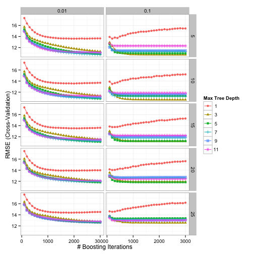
Using the "submodel trick" we evaluated 1600 tuning parameter combinations but only fit 600 models over all of the resamples. The optimal values were n.trees = 3000, interaction.depth = 3, shrinkage = 0.1, and n.minobsinnode = 10.

Random search yield optimal settings of n.trees = 2202, interaction.depth = 3, shrinkage = 0.02651, and n.minobsinnode = 9 also using 600 model fits for tuning.

Time-wise, the GBM GA took 8.46-fold longer to run compared to grid search and 9.95-fold longer than random search.

Test Set Results

Here are the results:

                 RMSE  Rsquared
 svm_ga      6.055410 0.9239437
 svm_grid    8.977140 0.8550142
 svm_random  7.877201 0.8853781
 gbm_ga     11.178473 0.7242996
 gbm_grid   11.223867 0.7145263
 gbm_random 11.130803 0.7253648
 

For one of the models, it was worth the trouble and time but not for the other. It is certainly possible that a larger number of random search tests would have achieved the same results and I think that I would put my effort there before using a GA to optimize. However, if I really need stellar performance, the GA is worth doing; the only cost is CPU cycles and that is usually limited by our patience.

Is this worth putting into caret? Probably but it is the kind of thing that would take some effort (and minor changes) to make it work across all different models. For example, self organizing maps have tuning parameters for the size of the two dimensions as well as the topology type (which is categorical). It doesn't make sense to evaluate networks with dimensions (3, 4) and also try (4, 3) since they are basically the same model. Also, encoding the categorical tuning parameters are not impossible but it might be tricky to do in an automated way. This would take some thought and, in the meantime, the code shown above works pretty well.

Simulated Annealing Feature Selection

As previously mentioned, caret has two new feature selection routines based on genetic algorithms (GA) and simulated annealing (SA). The help pages for the two new functions give a detailed account of the options, syntax etc.

The package already has functions to conduct feature selection using simple filters as well as recursive feature elimination (RFE). RFE can be very effective. It initially ranks the features, then removes them in sequence, starting with the least importance variables. It is a greedy method since it never backtracks to reevaluate a subset. Basically, it points itself in a single direction and proceeds. The main question is how far to go in that direction.

These two new functions, gafs and safs, conduct a global search over the feature set. This means that the direction of the search is constantly changing and may re-evaluate solutions that are similar to (or the same as) previously evaluated feature sets. This is good and bad. If a feature set is not easily "rankable" then it should do better than RFE. However, it will require a larger number of model fits and has a greater chance of overfitting the features to the training set.

I won't go over the details of GAs or SA. There are a lot of references on these and you can always check out Chapter 19 of our book. Also, since there were two previous blog posts about genetic algorithms, I'll focus on simulated annealing in this one.

To demonstrate I'll use the Alzheimer's disease data from Section 19.6 (page 502). It contains biomarker and patient demographic data that are being used to predict who will eventually have cognitive impairment. The original data contained instances for 333 subjects and information on 133 predictors.

In the book, we fit a number of different models to these data and conducted feature selection. Using RFE, linear discriminant analysis, generalized linear models and naive Bayes seemed to benefit from removing non-informative predictors. However, K-nearest neighbors and support vector machines had worse performance as RFE proceeded to remove predictors.

Wiht KNN, there is no model-based method for measuring predictor importance. In these cases, the rfe will use the area under the ROC curve for each individual predictor for ranking. Using that approach, here is the plot of KNN performance over subset sizes:

The values shown on the plot are the average area under the ROC curve measured using 5 repeats of 10-fold cross-validation. This implies that the full set of predictors is required. I should also note that, even with the entire predictor set, the KNN model did worse than LDA and random forests.

While RFE couldn't find a better subset of predictors, that does not mean that one doesn't exist. Can simulated annealing do better?

The code to load and split the data are in the AppliedPredictiveModeling package and you can find the markdown for this blog post linked at the bottom of this post. We have a data frame called training that has all the data used to fit the models. The outcome is a factor called Class and the predictor names are in a character vector called predVars. First, let's define the resampling folds.

Let's define the control object that will specify many of the important options for the search. There are a lot of details to spell out, such as how to train the model, how new samples are predicted etc. There is a pre-made list called caretSA that contains a starting template.

names(caretSA)
[1] "fit"            "pred"           "fitness_intern" "fitness_extern"
[5] "initial"        "perturb"        "prob"           "selectIter"    

These functions are detailed on the packages web page. We will make a copy of this and change the method of measuring performance using hold-out samples:

knnSA <- caretSA
knnSA$fitness_extern <- twoClassSummary

This will compute the area under the ROC curve and the sensitivity and specificity using the default 50% probability cutoff. These functions will be passed into the safs function (see below)

safs will conduct the SA search inside a resampling wrapper as defined by the index object that we created above (50 total times). For each subset, it computed and out-of-sample (i.e. "external") performance estimate to make sure that we are not overfitting to the feature set. This code should reproduce the same folds as those used in the book:

library(caret)
set.seed(104)
index <- createMultiFolds(training$Class, times = 5)

Here is the control object that we will use:

ctrl <- safsControl(functions = knnSA,
                    method = "repeatedcv",
                    repeats = 5,
                    ## Here are the exact folds to used:
                    index = index,
                    ## What should we optimize? 
                    metric = c(internal = "ROC",
                               external = "ROC"),
                    maximize = c(internal = TRUE,
                                 external = TRUE),
                    improve = 25,
                    allowParallel = TRUE)

The option improve specifies how many SA iterations can occur without improvement. Here, the search restarts at the last known improvement after 25 iterations where the internal fitness value has not improved. The allowParallel options tells the package that it can parallelize the external resampling loops (if parallel processing is available).

The metric argument above is a little different than it would for train or rfe. SA needs an internal estimate of performance to help guide the search. To that end, we will also use cross-validation to tune the KNN model and measure performance. Normally, we would use the train function to do this. For example, using the full set of predictors, this could might work to tune the model:

train(x = training[, predVars],
      y = training$Class,
      method = "knn",
      metric = "ROC",
      tuneLength = 20,
      preProc = c("center", "scale"),
      trControl = trainControl(method = "repeatedcv",
                               ## Produce class prob predictions
                               classProbs = TRUE,
                               summaryFunction = twoClassSummary,))

The beauty of using the caretSA functions is that the ... are available.

A short explanation of why you should care...

R has this great feature where you can seamlessly pass arguments between functions. Suppose we have this function that computes the means of the columns in a matrix or data frame:

mean_by_column <- function(x, ...) {
  results <- rep(NA, ncol(x))
  for(i in 1:ncol(x)) results[i] <- mean(x[, i], ...)
  results
  }

(aside: don't loop over columns with for. See ?apply, or ?colMeans, instead)

There might be some options to the mean function that we want to pass in but those options might change for different applications. Rather than making different versions of the function for different option combinations, any argument that we pass to mean_by_column that is not one it its arguments (x, in this case) is passed to wherever the three dots appear inside the function. For the function above, they go to mean. Suppose there are missing values in x:

example <- matrix(runif(100), ncol = 5)
example[1, 5] <- NA
example[16, 1] <- NA
mean_by_column(example)
[1]     NA 0.4922 0.4704 0.5381     NA

mean has an option called na.rm that will compute the mean on the complete data. Now, we can pass this into mean_by_column even though this is not one of its options.

mean_by_column(example, na.rm = TRUE)
[1] 0.5584 0.4922 0.4704 0.5381 0.4658

Here's why this is relevant. caretSA$fit uses train to fit and possibly tune the model.

caretSA$fit
function (x, y, lev = NULL, last = FALSE, ...) 
train(x, y, ...)

Any options that we pass to safs that are not x, y, iters, differences, or safsControl will be passed to train.

(Even further, any option passed to safs that isn't an option to train gets passed down one more time to the underlying fit function. A good example of this is using importance = TRUE with random forest models. )

So, putting it all together:

set.seed(721)
knn_sa <- safs(x = training[, predVars],
               y = training$Class,
               iters = 500,
               safsControl = ctrl,

               ## Now we pass options to `train` via "knnSA":               
               method = "knn",
               metric = "ROC",
               tuneLength = 20,
               preProc = c("center", "scale"),
               trControl = trainControl(method = "repeatedcv",
                                        repeats = 2,
                                        classProbs = TRUE,
                                        summaryFunction = twoClassSummary,
                                        allowParallel = FALSE))

To recap:

  • the SA is conducted many times inside of resampling to get an external estimate of performance.
  • inside of this external resampling loop, the KNN model is tuned using another, internal resampling procedure.
  • the area under the ROC curve is used to guide the search (internally) and to know if the SA has overfit to the features (externally)
  • in the code above, when safs is called with other options (e.g. method = "knn"),
    • safs passes the method, metric, tuneLength, preProc, and tuneLength, trControl options to caretSA$fit
      • caretSA$fit passes these options to train

After external resampling, the optimal number of search iterations is determined and one last SA is run using all of the training data.

Needless to say, this executes a lot of KNN models. When I ran this, I used parallel processing to speed things up using the doMC package.

Here are the results of the search:

knn_sa
Simulated Annealing Feature Selection

267 samples
132 predictors
2 classes: 'Impaired', 'Control' 

Maximum search iterations: 500 
Restart after 25 iterations without improvement (15.6 restarts on average)

Internal performance values: ROC, Sens, Spec
Subset selection driven to maximize internal ROC 

External performance values: ROC, Sens, Spec
Best iteration chose by maximizing external ROC 
External resampling method: Cross-Validated (10 fold, repeated 5 times) 

During resampling:
  * the top 5 selected variables (out of a possible 132):
    Ab_42 (96%), tau (92%), Cystatin_C (82%), NT_proBNP (82%), VEGF (82%)
  * on average, 60 variables were selected (min = 45, max = 75)

In the final search using the entire training set:
   * 59 features selected at iteration 488 including:
     Alpha_1_Antitrypsin, Alpha_1_Microglobulin, Alpha_2_Macroglobulin, Angiopoietin_2_ANG_2, Apolipoprotein_E ... 
   * external performance at this iteration is

       ROC       Sens       Spec 
     0.852      0.198      0.987 

The algorithm automatically chose the subset created at iteration 488 of the SA (based on the external ROC) which contained 59 out of 133 predictors.

We can also plot the performance values over iterations using the plot function. By default, this uses the ggplot2 package, so we can add a theme at the end of the call:

Each of the data points for the external fitness is a average of the 50 resampled ROC values. The most improvement was found in the first 200 iterations. The internal estimate is generally more optimistic than the external estimate. It also tends to increase while the external estimate is relatively flat, indicating some overfitting. The plot above indicates that less iterations might probably give us equivalent performance. Instead of repeating the SA with fewer iterations, the update function can be used to pick a different subset size.

Let's compare the RFE and SA profiles. For RFE and SA, the ROC values are averaged over the 50 resamples. In the case of SA, the number of predictors is also an average. For example, at iteration 100 of the SA, here is the subset size distribution across the 50 resamples:

Here are superimposed smoothed trend lines for the resampling profiles of each search method:

Recall that the same cross-validation folds were used for SA and RFE, so this is an apples-to-apples comparison. SA searched a smaller range of subset sizes over the iterations in comparison to RFE. The code here starts the initial subset with a random 20% of the possible features and tended to increase as the search continued and then stabilized at a size of about 55.

How does this predictor subset perform on the test data?

library(pROC)
roc(testing$Class,
    predict(knn_sa, testing)$Impaired,
    levels = rev(levels(testing$Class)))
Call:
roc.default(response = testing$Class, 
            predictor = predict(knn_sa, testing)$Impaired, 
            levels = rev(levels(testing$Class)))

Data: predict(knn_sa, testing)$Impaired in 48 controls 
      (testing$Class Control) <  18 cases (testing$Class 
      Impaired).
      
Area under the curve: 0.848

This is better than the test set results for the RFE procedure. Note that the test set AUC is much more in-line with the external estimate of the area under the ROC curve. The bad new is that we evaluated many more models than the RFE procedure and the SA process was slightly more than 11-fold slower than RFE to complete. Good things take time. Here is a parallel-coordinate plot of the individual resampling results, match by fold:

The difference is statistically signficant too:

summary(diff(rs, metric = "ROC"))
Call:
summary.diff.resamples(object = diff(rs, metric = "ROC"))

p-value adjustment: bonferroni 
Upper diagonal: estimates of the difference
Lower diagonal: p-value for H0: difference = 0

ROC 
    RFE      SA     
RFE          -0.0504
SA  8.02e-06        

The genetic algorithm code in gafs has very similar syntax to safs and also has pre-made functions.

The knitr file for these analyses can be found here

New Version of caret on CRAN

A new version of caret is on CRAN.

ga_rf_profile.png

Some recent features/changes:

  • The license was changed to GPL >= 2 to accommodate new code from the GA package.
  • New feature selection functions gafs and safs were added, along with helper functions and objects, were added. The package HTML was updated to expand more about feature selection. I'll talk more about these functions in an upcoming blog post.
  • A reworked version of nearZerVar based on code from Michael Benesty was added the old version is now called nzv that uses less memory and can be used in parallel.
  • sbfControl now has a multivariate option where all the predictors are exposed to the scoring function at once.
  • Several regression simulation functions were added: SLC14_1, SLC14_2, LPH07_1 and LPH07_2
  • For the input data x to train, we now respect the class of the input value to accommodate other data types (such as sparse matrices).
  • A function update.rfe was added.

Recently added models:

  • From the adabag package, two new models were added: AdaBag and AdaBoost.M1.
  • Weighted subspace random forests from the wsrf package was added.
  • Additional bagged FDA and MARS models were added (model codes bagFDAGCV and bagEarthGCV) were added that use the GCV statistic to prune the model. This leads to memory reductions during training.
  • Brenton Kenkel added ordered logistic or probit regression to train using method = "polr" from MASS
  • The adaptive mixture discriminant model from the adaptDA package
  • A robust mixture discriminant model from the robustDA package was added.
  • The multi-class discriminant model using binary predictors in the binda package was added.
  • Ensembles of partial least squares models (via the enpls package) was added.
  • plsRglm was added.
  • From the kernlab package, SVM models using string kernels were added: svmBoundrangeString, svmExpoString, svmSpectrumString
  • The model code for ada had a bug fix applied and the code was adapted to use the "sub-model trick" so it should train faster.