Previously, I talked about genetic algorithms (GA) for feature selection and illustrated the algorithm using a modified version of the GA R package and simulated data. The data were simulated with 200 non-informative predictors and 12 linear effects and three non-linear effects. Quadratic discriminant analysis (QDA) was used to model the data. The last set of analyses showed, for these data, that:
- The performance of QDA suffered from including the irrelevant terms.
- Using a resampled estimate area under the ROC curve resulted in selection bias and severely over-fit to the predictor set.
- Using a single test set to estimate the fitness value did marginally better model with an area under the ROC curve of 0.622.
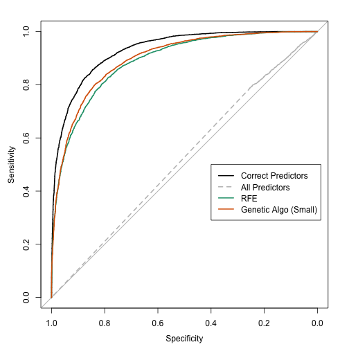
- Recursive feature elimination (RFE) was also used and found a much better predictor subset with good performance (an AUC of 0.885 using the large-sample data set).
For the genetic algorithm, I used the default parameters (e.g. crossover rate, mutation probability etc). Can we do better with GA's?
One characteristic seen in the last set of analyses is that, as the number of irrelevant predictors increases, there is a gradual decrease in the fitness value (although the true performance gets worse). The initial population of chromosomes for the GA is based on simple random sampling, which means that each predictor has about a 50% chance of being included. Since our true subset is much smaller, the GA should favor smaller sets and move towards cases with fewer predictors... except that it didn't. I think that this didn't happen because the of two reasons:
The increase in performance caused by removing a single predictor is small. Since there is no "performance cliff" for this model, the GA isn't able to see improvements in performance unless a subset is tested with a very low number of predictors.
Clearly, using the evaluation set and resampling to measure the fitness value did not penalize larger models enough. The plots of these estimates versus the large sample estimates showed that they were not effective measurements. Note that the RFE procedure did not have this issue since the feature selection was conducted within the resampling process (and reduced the effect of selection bias).
Would resampling the entire GA process help? It might but I doubt it. It only affects how performance is measured and does not help the selection of features, which is the underlying issue. I think it would result in another over-fit model and all that the resampling would do would be to accurately tell when the model begins to over-fit. I might test this hypothesis in another post.
There are two approaches that I'll try here to improve the effectiveness of the GA. The first is to modify the initial population. If we have a large number of irrelevant predictors in the model, the GA has difficultly driving the number of predictors down. However, would the converse be true? We are doing feature selection. Why not start the GA with a set of chromosomes with small predictor sets. Would the algorithm drive up the number of predictors or would it see the loss of performance and keep the number small?
To test this, I simulated the same data sets:
set.seed(468)
training <- twoClassSim(500, noiseVars = 100,
                        corrVar = 100, corrValue = 0.75)
testing <- twoClassSim(500, noiseVars = 100,
                       corrVar = 100, corrValue = 0.75)
large <- twoClassSim(10000, noiseVars = 100,
                     corrVar = 100, corrValue = 0.75)
realVars <- names(training)
realVars <- realVars[!grepl("(Corr)|(Noise)", realVars)]
cvIndex <- createMultiFolds(training$Class, times = 2)
ctrl <- trainControl(method = "repeatedcv",
                     repeats = 2,
                     classProbs = TRUE,
                     summaryFunction = twoClassSummary,
                     allowParallel = FALSE,
                     index = cvIndex)
The ga function has a parameter for creating the initial population. I'll use one that produces chromosomes with a random 10% of the predictors.
initialSmall <- function(object, ...)
{
    population <- sample(0:1,
                         replace = TRUE,
                         size = object@nBits * object@popSize,
                         prob = c(0.9, 0.1))
    population <- matrix(population,
                         nrow = object@popSize,
                         ncol = object@nBits)
    return(population)
}
Then I'll run the GA again (see the last post for more explanation of this code).
ROCcv <- function(ind, x, y, cntrl)
{
    library(caret)
    library(MASS)
    ind <- which(ind == 1)
    ## In case no predictors are selected:
    if (length(ind) == 0)  return(0)
    out <- train(x[, ind], y,
                 method = "qda",
                 metric = "ROC",
                 trControl = cntrl)
    ## Return the resampled ROC value
    caret:::getTrainPerf(out)[, "TrainROC"]
}

set.seed(137)
ga_small_cv <- ga(type = "binary",
                  fitness = ROCcv,
                  min = 0, max = 1,
                  maxiter = 400,
                  population = initialSmall,
                  nBits = ncol(training) - 1,
                  names = names(training)[-ncol(training)],
                  x = training[, -ncol(training)],
                  y = training$Class,
                  cntrl = ctrl,
                  keepBest = TRUE,
                  parallel = FALSE)
The genetic algorithm converged on a subset size of 14 predictors. This included 5 of the 10 linear predictors, 0 of the non-linear terms and both of the terms that have an interaction effect in the model. The trends were: