In Chapter 11, equivocal zones were briefly discussed. The idea is that some classification errors are close to the probability boundary (i.e. 50% for two class outcomes). If this is the case, we can create a zone where we the samples are predicted as "equivocal" or "indeterminate" instead of one of the class levels. This only works if the model does not incorrectly classify samples with complete (but wrong) confidence.
In molecular diagnostics, many assays are required to have these zones for FDA approval and great care goes into their determination. If the assay returns an equivocal result, a recommendation would be made to repeat the assay or to obtain another sample.
Does this actually work with a classification model? How would we do it in R?
To illustrate this, I will use the two-class simulation system outlined here. For example:
Let's fit a random forest model using the default tuning parameter value to get a sense of the baseline performance. I'll calculate a set of different classification metrics: the area under the ROC curve, accuracy, Kappa, sensitivity and specificity.
p <- ncol(training) - 1

fiveStats <- function(...) c(twoClassSummary(...), defaultSummary(...))

ctrl <- trainControl(method = "cv",
                     summaryFunction = fiveStats,
                     classProbs = TRUE)

set.seed(721)
rfFit <- train(Class ~ ., data = training,
                method = "rf",
                metric = "ROC",
                tuneGrid = data.frame(.mtry = floor(sqrt(p))),
                ntree = 1000,
                trControl = ctrl)
> rfFit
1000 samples
  15 predictors
   2 classes: 'Class1', 'Class2'

No pre-processing
Resampling: Cross-Validation (10 fold)

Summary of sample sizes: 900, 900, 900, 900, 900, 900, ...

Resampling results

  ROC    Sens   Spec   Accuracy  Kappa  ROC SD  Sens SD  Spec SD  Accuracy SD
  0.924  0.856  0.817  0.837     0.673  0.0329  0.0731   0.0561   0.0536
  Kappa SD
  0.107

Tuning parameter 'mtry' was held constant at a value of 3
We will fit the same model but performance is only measured using samples outside the zone:
eZoned <- function(...)
{
  ## Find points within 0.5 +/- zone
  buffer <- .10
  preds <- list(...)[[1]]
  inZone <- preds$Class1 > (.5 - buffer) & preds$Class1 < (.5 + buffer)
  preds2 <- preds[!inZone,]
  c(twoClassSummary(preds2, lev = levels(preds2$obs)),
    defaultSummary(preds2),
    ## We should measure the rate in which we do not make
    ## a prediction.
    Reportable = mean(!inZone))
}

ctrlWithZone <- trainControl(method = "cv",
                             summaryFunction = eZoned,
                             classProbs = TRUE)
set.seed(721)
rfEZ <- train(Class ~ ., data = training,
              method = "rf",
              metric = "ROC",
              tuneGrid = data.frame(.mtry = floor(sqrt(p))),
              ntree = 1000,
              trControl = ctrlWithZone)
> rfEZ
1000 samples
  15 predictors
   2 classes: 'Class1', 'Class2'

No pre-processing
Resampling: Cross-Validation (10 fold)

Summary of sample sizes: 900, 900, 900, 900, 900, 900, ...

Resampling results

  ROC   Sens   Spec   Accuracy  Kappa  Reportable  ROC SD  Sens SD  Spec SD
  0.96  0.917  0.891  0.905     0.808  0.767       0.024   0.0483   0.0668
  Accuracy SD  Kappa SD  Reportable SD
  0.0507       0.102     0.0655

Tuning parameter 'mtry' was held constant at a value of 3
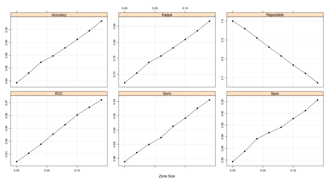
So by failing to predict about 23% of the samples, we were able to achieve a good boost in performance. What would happen if we change the zone size? The same procedure what used with zones up to +/- 0.14 and here are the results for the various metrics:
There is an improvement in each of the measures as long as we are willing to accept an increasing proportion of indeterminate results. Does this replicate in the test set?
rfPred <- predict(rfFit, testing)
rfProb <- predict(rfFit, testing, type = "prob")[, "Class1"]
rfPred <- data.frame(obs = testing$Class,
                     pred = rfPred,
                     Class1 = rfProb)

fiveStats(rfPred, lev = levels(rfPred$obs))
eZoned(rfPred, lev = levels(rfPred$obs))
> fiveStats(rfPred, lev = levels(rfPred$obs))
      ROC      Sens      Spec  Accuracy     Kappa
0.9378583 0.8518519 0.8543478 0.8530000 0.7047244
> eZoned(rfPred, lev = levels(rfPred$obs))
       ROC       Sens       Spec   Accuracy      Kappa Reportable
 0.9678054  0.9361702  0.9239437  0.9305913  0.8601139  0.7780000

